Exact Sampling with Coupled Markov Chains and Swendsen-Wang Cluster Sampling of the Ising Model

For high-dimensional problems, widely used random sampling methods include Markov Chain Monte Carlo (MCMC) methods like the Metropolis-Hastings method, Gibbs sampling, and slice sampling. One can run an ergodic, i.e. irreducible aperiodic, Markov chain whose stationary distribution is the desired distribution of the set. These methods are guaranteed to produce samples from a target density asymptotically, as long as the Markov chain has converged to the equilibrium, or stationary, distribution $\pi$.

Naturally, the principal concern with these methods is how many iterations $M$ the Markov chain should be run to reach the stationary distribution. This can often be very difficult to determine. Presenting a method that solves for this during runtime, James Propp and David Wilson introduced exact sampling with coupled Markov chains in 1996. Propp and Wilson’s exact sampling method, also known as perfect simulation or coupling from the past, depends on three key ideas: coalesence of coupled Markov chains, coupling from the past, and monotonicity.

Introduced by Robert Swendsen and Jian-Sheng Wang in 1987, the Swendsen-Wang (SW) algorithm was initially designed to address a well-known, critical slow-down in effective sampling that occurs for the Ising/Potts model. Specifically, near critical temperatures in which phase transitions occur, there is a dramatic increase in the number of samples required to obtain valid random samples from the model. The key feature of the Swendsen-Wang algorithm was the random cluster model. The random cluster model is a representation of the Ising/Potts model through percolation models of connecting bonds. The SW algorithm has since been generalized by Adrian Barbu and Song-Chun Zhu in 2005 to arbitrary sampling probabilities. This requires interpreting the SW algorithm in a Metropolis-Hastings fashion by computing acceptance probabilities of proposed Monte Carlo moves.

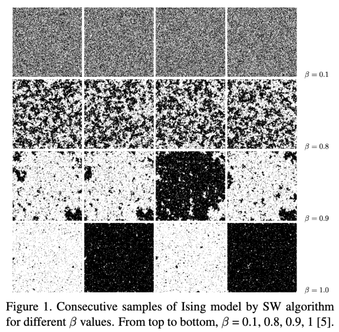
For various values of $\beta$, we can observe consecutive samples of the Ising model obtained by the SW algorithm for an example lattice 256x256:

For $\beta = \textbf{0.84}$, we display the coalesence of the white and black coupled Markov chains. They coalesce at $\tau = \textbf{887}$ sweeps of the exact Gibbs sampling method.

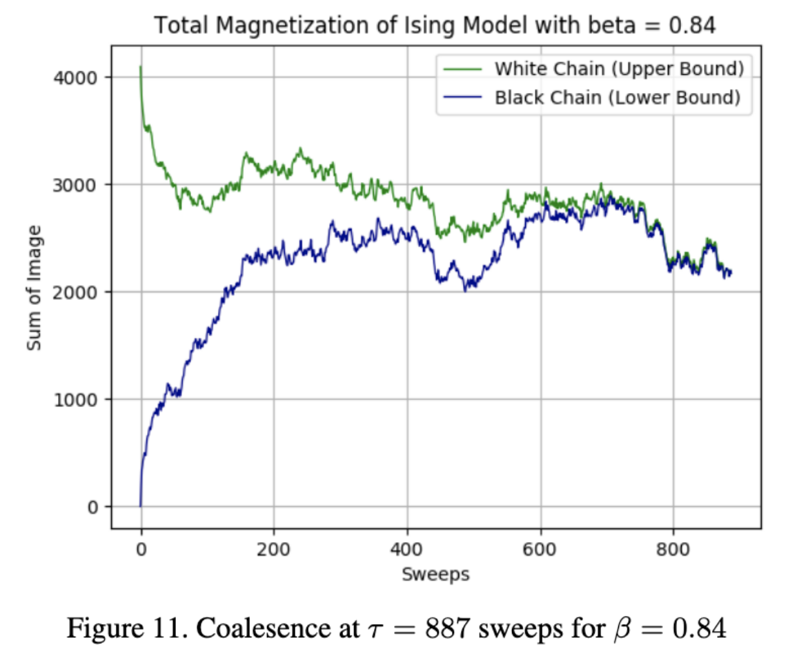
Increasing $\beta$ from 0.83 to 0.84, a seemingly small transition, caused a roughly 2.5x increase in the number of sweeps necessary for coalesence. Roughly at this value of $\beta = 0.84$, the Ising model undergoes a phase transition. The sampling demands have increased greatly for just a small increase in the ferro-magnetism strength $\beta$.

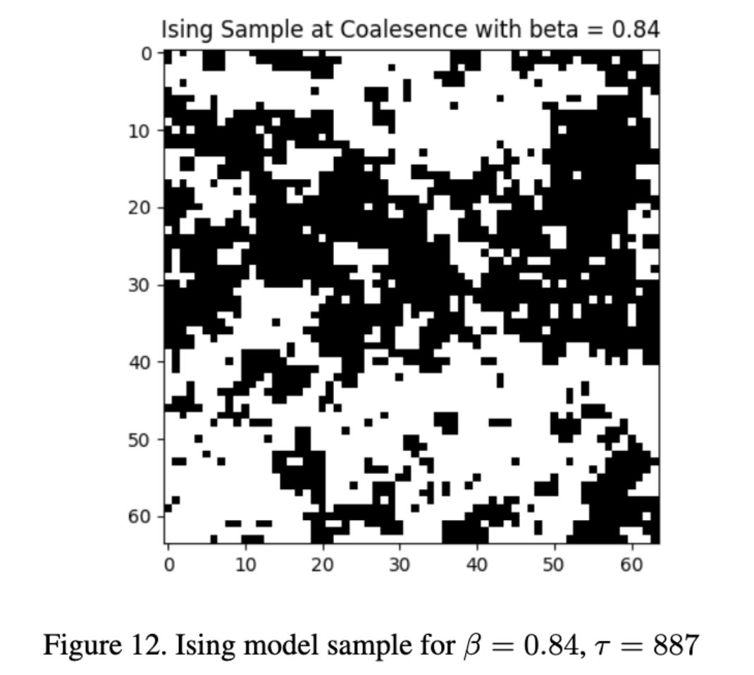
Below we display a sample of the Ising model at coalesence for $\beta = 0.84$ and $\tau = 887$.

We can display a plot of the coalesence times $\tau$ for each of the values of $\beta$ = [$\textbf{0.5}$, $\textbf{0.6}$, $\textbf{0.7}$, $\textbf{0.8}$, $\textbf{0.83}$, $\textbf{0.84}$, $\textbf{0.85}$, $\textbf{0.9}$] used in the Ising model.

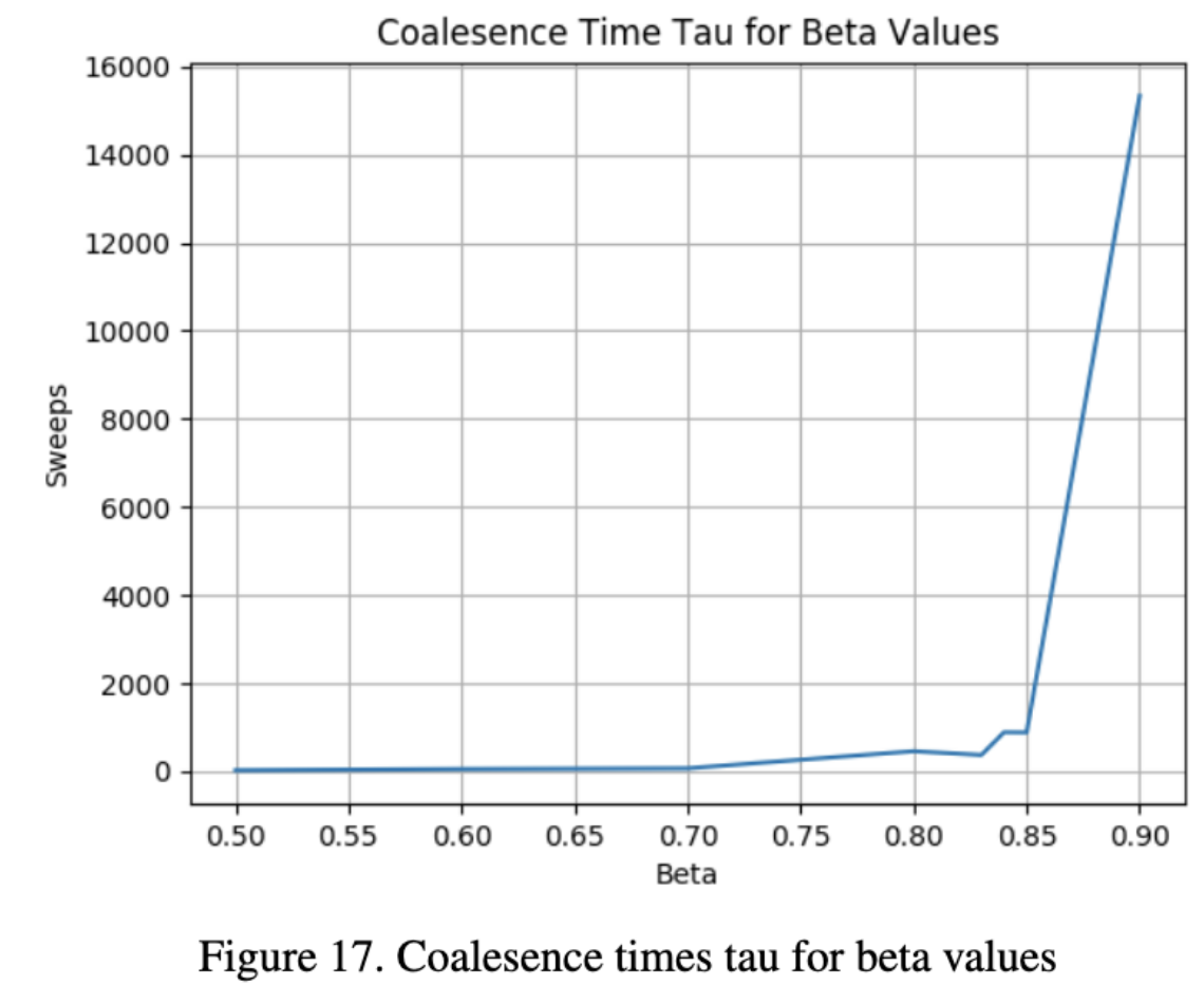
This final plot of $\tau$ over $\beta$ shows that at about $\beta = 0.85$, a phase transition occurs which causes a critical slow-down in the sweeps required for coalesence. In effect, many more sweeps of the Gibbs sampler will be necessary for $\beta$ values larger than 0.85 to ensure we have accurate random samples of the distribution.

Convergence with cluster sampling is determined by whether $H(X)$, the sufficient statistics of $X$ that measures the length of total boundaries (or cracks), converges to a constant value $h$ over time. We plot the sufficient statistics $H(X)$ over sweeps for $\beta = \textbf{0.84}$. We do this for both initializations, the constant image and checkerboard image. We placed red markers for the times at which the Markov chains converged to the sufficient statistic $h_3^* = \textbf{0.1966}$ given this beta value.

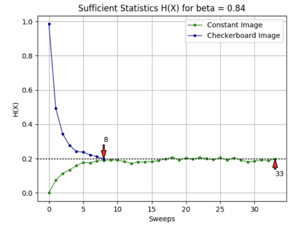
Similar to the results seen with exact sampling, notice how a larger value of $\beta$ increases the sweeps $\tau$ required for convergence. This is to be expected, as an increase in the ferro-magnetism strength $\beta$ more strongly configures neighboring vertices to have similar labels, encouraging clustering and slowing the mixing time of the chains.

We plot the average sizes of the connected components (CP), or the number of pixels flipped together at each sweep, for each of the three values $\beta = $ 0.6, 0.8, and 0.84.

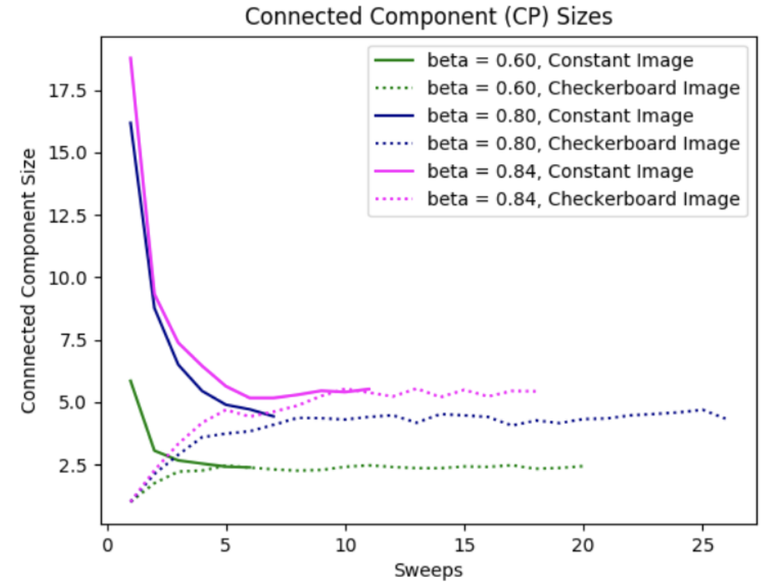
The outstanding observation is that as $\beta$ increases from 0.6 to 0.84, the average CP size also increases. This is intuitive, as we know that a stronger ferro-magnetic strength $\beta$ more strongly promotes neighboring vertices to have similar labels and hence it promotes clustering. With larger clusters on average, the average CP size, or the average number of pixels flipped together at each sweep, will certainly be larger.

It also seems that larger values of $\beta$ correspond to greater variation in average CP sizes. The value $\beta = 0.84$ caused the most variation and the largest number of sweeps necessary for the constant and checkerboard images to converge to roughly the same CP size per sweep. This is also reasonable, as stronger $\beta$ values promote stronger clustering, which promotes the formation of more and larger clusters, which in turn produces greater variation in cluster sizes.

The Swendsen-Wang clustering method is limited in two ways we have not mentioned. First, it is only valid for the Ising and Potts models. Second, it requires that the number of labels, or colors, $L$ be known. In applications such as image analysis, $L$ may represent the number of objects (or image regions) that have to be inferred from input data.

For future work, I would like to explore data-driven Markov Chain Monte Carlo methods, which do not require that the number of labels $L$ be known. Utilizing a Bayesian statistical framework, data-driven Markov Chain Monte Carlo methods perform image segmentation and hence labeling in a purely data-driven manner.